Examples

Estimate Risk Neutral Density with risk_neutral_density.Calculator

Use the class risk_neutral_density.Calculator in order to estimate the RND via Rookley’s Method. Set the logging level to INFO if status reports are of interest.

import os
import pandas as pd
from matplotlib import pyplot as plt
from spd_trading import risk_neutral_density as rnd

RND_TESTDATA_FILENAME = os.path.join(".", "examples", "data", "rnd_input_data.csv")
rnd_input_data = pd.read_csv(RND_TESTDATA_FILENAME)
evaluation_day = "2020-03-05"    # known from data processing
evaluation_tau = 8               # known from data processing

RND = rnd.Calculator(
    data=rnd_input_data,
    tau_day=evaluation_tau,
    date=evaluation_day,
    sampling="slicing",
    n_sections=15,
    loss="MSE",
    kernel="gaussian",
    h_m=0.088,                   # set None if bandwidth unknown
    h_k=215.068,                 # if unknow, use `localpoly.bandwidth_cv`
    h_m2=0.036,                  # for bandwidth optimization
)
RND.get_rnd()

RndPlot = rnd.Plot()             # Rookley Method algorithm plot
fig_method = RndPlot.rookleyMethod(RND)

plt.show()

Estimate Historical Density with historical_density.Calculator

Use the class historical_density.Calculator in order to estimate the HD via Monte Carlo Simulation on a GARCH Model of the historical data. Set the logging level to INFO if status reports are of interest.

import os
import pandas as pd
from matplotlib import pyplot as plt
from spd_trading import historical_density as hd

HD_TESTDATA_FILENAME = os.path.join(".", "examples", "data", "hd_input_data.csv")

hd_input_data = pd.read_csv(HD_TESTDATA_FILENAME)
evaluation_day = "2020-03-05"    # known from data processing
evaluation_tau = 8               # known from data processing
evaluation_S0 = hd_input_data.loc[
    hd_input_data.date_str == evaluation_day, "price"
].item()                         # either take from index or replace by other value

HD = hd.Calculator(
    data=hd_input_data,
    S0=evaluation_S0,
    garch_data_folder=os.path.join(".", "examples", "data"),
    tau_day=evaluation_tau,
    date=evaluation_day,
    n_fits=400,
    simulations=5000,
    overwrite_model=True,
    overwrite_simulations=True,
)
HD.get_hd(variate=True)

HdPlot = hd.Plot()
fig_denstiy = HdPlot.density(HD)

plt.show()

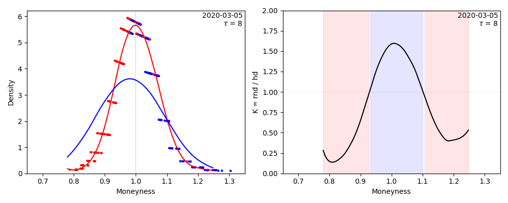
Calculate and Plot Kernel with kernel.Plot

Estimate RND and HD as shown in the previous examples, then use kernel.Plot to calculate the Kernel and plot the result. Use the previous examples to train instances of RND and HD. Set the logging level to INFO if status reports are of interest.

import os
import pandas as pd
from matplotlib import pyplot as plt
from spd_trading import kernel as ker

Kernel = ker.Calculator(
    tau_day=evaluation_tau,
    date=evaluation_day,
    RND=RND,
    HD=HD,
    cut_tail_percent=0.02
)
Kernel.calc_kernel()
Kernel.calc_trading_intervals()

TradingPlot = ker.Plot(x=0.35)  # kernel plot - comparison of rnd and hd
fig_strategy = TradingPlot.kernelplot(Kernel)