Theoretical Background
In the setting of a perfect financial market, the arbitrage free price of an option is derived from its expected payoff at maturity \(T\) (under the risk neutral measure \(\mathbb{Q}\)), discounted to the time of interest \(t\) via the riskfree interest rate \(r\) that one would get if invested in the underlying directly. 1
Where we call \(q_{t}(S_T)\) the Risk Neutral Density (RND) or State Price Density of the underlying \(S_T\) at time \(t\), which is derived from the option prices of the underlying in the market under the risk neutral measure \(\mathbb{Q}\).
Under the physical measure \(\mathbb{P}\), the “true” measure, the price of the option can not easily be expressed in the same way, since the discounted price process is not a martingale under this measure.
The Radon-Nykodym Lemma which evolves from the more general Girsanov Theorem states, how a change from \(\mathbb{P}\) to \(\mathbb{Q}\) is possible:
Let \(\mathbb{P}\) and \(\mathbb{Q}\) be equivalent measures and \(X_t\) and \(\mathcal{F}_t\)-adapetd process, then
where we define the Radon-Nikodym derivative of \(\mathbb{Q}\) with respect to \(\mathbb{P}\) to be \(K_t := \mathbb{E}_\mathbb{P}\left[ \frac{d \mathbb{Q}}{d \mathbb{P}} \rvert \mathcal{F}_t \right]\).
The price of the option can now be expressed via the physical density \(\mathbb{P}\) as:
Where we call \(p_{t}(S_T)\) the Historical Density (HD) or Empirical Density of the underlying \(S_T\) at time \(t\), which is dericed from the timeseries of historical values of the underlying itself.
Risk Neutral Density
The Risk Neutral Density (RND) is derived from the options that are offered on the market. On one trading day, options with different maturity \(T\) are offered. A set of options with the same maturity consists of options with different strike prices \(K\) (and therefore different price of option, different implied volatility).
These information are sufficient to use a semi-parametric approach to estimate the Risk Neutral Density. It uses the results of Breeden and Litzenberger 2, where Arrow-Debreu prices are replicated using butterfly spreads on Europeak options. mytodo{add how the replication strategy works?}
As an end result they find:
Rookley’s Method
Rookley found an analytical solution to the equation above by representing the call-price by the Black-Scholes call option pricing formula 3.
The analytical solution is quite lengthy, therefore the equations are not listed here.
One crucial point is, that in order to use Rookely’s Method, we need the volatility smile and its first and second derivatives
\((\sigma(M), \frac{\partial \sigma(M)}{\partial M}, \frac{\partial^2 \sigma(M)}{\partial M^2})\).
In practice, we will estimate them with Local Polynomial Regression (install package: localpoly (documentation))
The steps of the algorithm are shown in the following graphic.

Historical Density
GARCH(1,1) Model
The Historical Density (HD) is derived from the timeseries of historical returns of the underlying. A simple but sufficient model is the GARCH(1,1) model, since it accounts for the heteroscedasticity of the timeseries 4.
We define the series of log returns as:
where \(S_t\) is the value of the underlying at time \(t\). In the GARCH(1,1) model, the log return \(X_t\) is expressed as the time-varying variance parameter \(\sigma_t^2\) multiplied by a i.i.d random innovation \(z_t\), the random shock.
The variance parameter itself is a weighted combination of the previous variance and the previous return. It therefore is called conditional variance, since it depends on all previous returns.
The GARCH(1,1) model has the following form:
After fitting the model to the data, the model is used to simulate many potential paths of the underlying. The HD is obtained by Kernel Density Estimation on these paths.
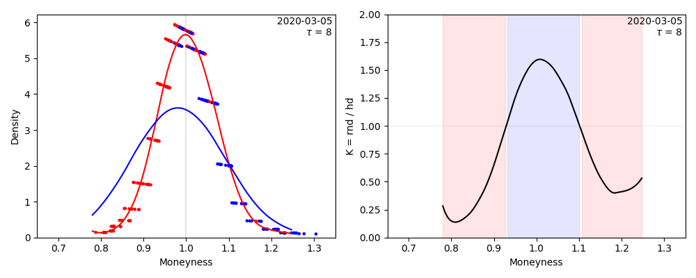
Trading on Differences between RND and HD
A Pricing Kernel can be calculated, which is used to determine trading strategies.
The Kernel is the quotient of Risk Neutral Density divided by Historical Density and therefore represents discrepancies in the future’s price distribution by the market (RND - red curve) vs. the historical data (HD - blue curve) 5, 6:
Resources:
- 1
The Valuation of Options for Alternative Stochastic Processes - Cox, John C. and Ross, Stephen A. - 1976
- 2
Prices of State-Contingent Claims Implicit in Option Prices - Breeden, Douglas T. and Litzenberger, Robert H. - 1978
- 3
Option Pricing and Risk Management - Rookley, Cameron - 1997
- 4
Estimation of Tail-Related Risk Measures for Heteroscedastic Financial Time Series: An Extreme Value Approach - McNeil, Alexander J. and Frey, Ruediger - 2000
- 5
Do Option Markets Correctly Price the Probabilities of Movement of the Underlying Asset? - Aı̈t-Sahalia, Y. Wang, and F. Yared - 2001
- 6
“Trading on Deviations of Implied and Historical Densities” in Applied Quantitative Finance - K. W. Haerdle, O. J. Blaskowitz and P. Schmidt - 2002